10X more data, same 4 seconds: single-query scaling in Redpanda SQL on 1 TB

When it comes to a distributed SQL engine, people always ask, "Does this scale?" and they usually mean two things: Do everyday dashboard queries stay fast as data grows, and can I speed up my heaviest, full-database queries by adding hardware?

For the unfamiliar, Redpanda SQL is a Postgres-compatible analytical query engine that joins live-streaming topics and historical Apache Iceberg™ tables. To achieve this, it uses “bridge queries” to read live records and historical records in a single SQL statement, then deliver a unified result.

In this benchmark, our engineering team asked those same questions and put Redpanda SQL to the test using a real-world, highly skewed dataset: NYC Taxi trip records, scaled from 100 GB (0.61 billion rows) all the way up to 1 TB (6.07 billion rows).

The TL;DR of what we found:

• What matters for latency is the data actually scanned, not the data retained: When filtering by a specific timeframe, the query took about 4 to 5 seconds whether the engine was searching through 100 GB of total data or 1 TB of total data, while a full scan of the same data grows from 17 s to 181 s.
• Heavy queries scale with hardware: For complex, full-database queries that must scan every row, throwing more servers (nodes) at the problem directly solves it. A heavy grouping query dropped from taking about 5 minutes (298 seconds) on one node to just 43 seconds on eight nodes.
• A new sizing rule: You no longer need to size your compute cluster based on your total data volume. Instead, you size it for your single heaviest analytical query, because your standard, time-bound dashboard queries will be efficient by default.

Now let’s get into how we arrived at these conclusions, the one caveat we found, and what it all means for Redpanda SQL users.

The real scaling question

To be clear, when someone asks, "Does your engine scale?"—they usually mean one of two things:

1. Can one heavy query go faster if I add machines?
2. Can I run more queries at once if I add machines?

The first is strong scaling in the classic sense: fix the work, add resources, and see how far the speedup goes before the serial fraction caps it. The second is throughput scaling, a capacity question about independent queries sharing a cluster. 

The two have different limits and different sizing math, which is why TPC-H measures them separately as a single-stream Power test and a multi-stream Throughput test. This post is about the first one, because for an analytical engine it decides whether your heaviest query is feasible at all on a given cluster.

There’s also a question that the scaling framing skips entirely: how much data does the query have to touch in the first place? That turns out to be the bigger lever, and it's where streaming plus Iceberg does something the stream alone can't.

Why we grew a real dataset

Strong scaling only gets interesting when the work actually needs multiple machines. A dataset that fits in one node's RAM measures caches, not distribution. Synthetic data has a different problem: real analytical workloads are skewed and heavy-tailed, with a few keys dominating, while generated data tends to be uniform. Skew stresses distributed aggregation, since it determines how evenly work and memory divide across nodes.

We started with the public NYC TLC Yellow Taxi trip records and grew them. The base is the cleaned 2016-onward slice (~0.61 B rows ≈ 100 GB). Larger sizes are built by replicating it with a per-replica time shift: each copy is the full dataset with every timestamp moved forward by N years, so the history extends continuously instead of duplicating the same instants. The per-record distribution and temporal ordering stay real while the corpus reaches 500 GB and 1 TB (3.03 / 6.07B rows). To be precise about provenance: everything is grown from real data, but the volume above 100 GB is extrapolated by replication. This matters for one result below.

So how does the data get queried? Each dataset is produced into its own Redpanda topic over the Apache Kafka^® API. Redpanda Streaming continuously materializes the topic to Parquet in S3 as an Iceberg table, cataloged in AWS Glue, and writes per-column min/max statistics into the Iceberg manifests as it goes. Redpanda SQL queries the topic through a transparent catalog that unifies the streaming tail (recent records not yet materialized) with its Iceberg copy (taxi_t=>trips in the SQL below references the trips topic through the taxi_t catalog). 

We ran every query after materialization had fully caught up, so the tail was empty and all rows were read from Iceberg. The engine reads Parquet from object storage, so above roughly 500 GB the working set exceeds cluster RAM. Nodes are m7i.2xlarge (8 vCPU / 32 GiB), so 1 - 8 nodes means 8 - 64 vCPU. All times are warm: a warm-up run first populates OS and storage caches, then we report the mean of 2 timed runs. Run-to-run spread is within a few percent for the long full-corpus queries; the ~4 s pushdown query varies up to ~20% between runs. Cold-start is out of scope here. The first query after idle additionally pays object-storage read latency.

Result 1: queries pruned by statistics

Start with a common analytical question, totals for a time window:

SELECT COUNT(*), SUM(total_amount)
  FROM taxi_t=>trips
 WHERE pickup_datetime >= '2023-01-01'
   AND pickup_datetime <  '2024-01-01';

You can run this against a raw Kafka topic, since any consumer can read every record and filter. But the log itself can only prune by offset and by record timestamp. A predicate on an arbitrary column like pickup_datetime (the event time inside the payload) has no index to seek on, so answering it means reading every record ever written.

The Iceberg bridge changes that. Because Redpanda writes column statistics into the manifests, Redpanda SQL reads each data file's pickup_datetime min/max and skips files whose range can't overlap 2023 before reading a byte of them. On our 1 TB corpus, the 2023 filter examines 4,961 data files and reads just 76 of them, about 1.1 GB. The rest are pruned at planning time. This works because records were produced in pickup_datetime order, so each data file spans a narrow time range. A naive load that interleaves years gives every file a wide range, and then nothing prunes.

The charts below show the result.

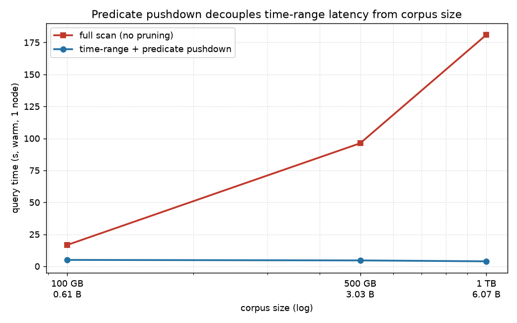
The pruned query sits at ~4–5 s across a 10X range of total data while the full scan grows roughly linearly, 17 s to 181 s.

‍One caveat about this chart: because we grow the corpus by time-shifting replicas, the year 2023 exists only in the base replica, so the 2023 filter matches the same ~1 GB slice at every corpus size. What the experiment isolates is that the cost of pruning stays negligible even as the candidate file count grows 10X: the planner discards thousands of non-overlapping files cheaply, and latency tracks the matched slice. 

In a deployment where the queried window itself accumulates more data, that slice would grow, and the latency with it. The durable claim is the mechanism. Query cost follows the amount of data scanned, not the amount retained, which is the property that makes long retention affordable. And it exists only because the topic is materialized to an Iceberg table with statistics the engine plans against.

Result 2: queries that benefit from more nodes

Not every query prunes. Here are two aggregations that must read the whole corpus. The first groups trips and revenue by payment type—just five groups. The second rolls up trips and revenue per hour per pickup zone and produces millions of distinct groups:

-- light: low-cardinality group-by (Q2)
SELECT payment_type, COUNT(*), AVG(trip_distance), SUM(fare_amount)
  FROM taxi_t=>trips GROUP BY payment_type ORDER BY payment_type;

-- heavy: high-cardinality rollup, millions of groups (Q7)
SELECT COUNT(*) AS groups, SUM(n) AS total
  FROM (SELECT date_trunc('hour', pickup_datetime) AS hr,
               pickup_location_id AS zone,
               COUNT(*) AS n, SUM(total_amount) AS revenue
          FROM taxi_t=>trips GROUP BY 1, 2) s;

When there’s no predicate to prune on, the lever is the cluster. Redpanda SQL is shared-nothing compute over shared object storage: adding nodes redistributes scan and aggregation work, and no data has to migrate between nodes. Swept across 1 - 8 nodes at 1 TB:

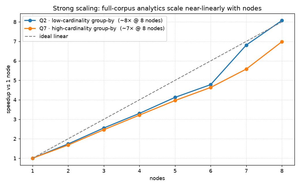
The heavy rollup drops from 298 s to 43 s, a 7X speedup on 8 nodes. For a query producing millions of groups, that’s close to the ideal diagonal.

The light group-by comes in at ~8X - linear within run-to-run noise. Either way, the shape is what matters: for scan-dominated aggregations, doubling the cluster roughly halves the time, all the way to 8 nodes.

The pushdown query on that same chart barely moves, going from 4.8 s to 3.3 s across all eight cluster sizes. This is expected. Once pruning has cut the read to ~1 GB, there’s almost nothing left to parallelize, and the win came from the Iceberg statistics rather than from the cluster.

A scope note: this sweep is at 1 TB and covers scan and group-by workloads. Join and window queries shuffle more data between nodes and can scale less cleanly. They were out of scope for this run, so read "near-linear" as a statement about scans and aggregations rather than a universal guarantee.

Result 3: memory shards with the cluster

The heavy rollup doubles as a memory probe. A high-cardinality GROUP BY builds a hash table sized to the number of distinct keys, and in a shared-nothing engine that state is partitioned across nodes, so per-node peak memory falls as the cluster grows. (Per-node memory below was profiled on our earlier multi-node sizing runs; the sharding behavior is the point, not the exact bytes.)

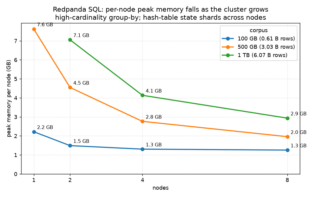
Roughly the total hash-table state ÷ nodes, with two qualifications. Each node carries a fixed per-process baseline, so the drop is somewhat shallower than a pure ÷N. And the ÷N estimate assumes even key distribution: with skewed keys, hot partitions land on some nodes and the per-node peak exceeds the average, so you have to size for the busiest node rather than the mean. 

‍Note: The grouping key here is (hour, zone), which spreads far more evenly than a raw per-trip key would; that's why the curve looks clean.

All of this matters because Redpanda SQL does not spill to disk. Working state lives in memory, and exceeding per-node RAM is a hard failure rather than a graceful slowdown. The upside is that adding nodes buys lower latency and lower per-node memory at the same time, which makes scale-out with some skew headroom the right lever for heavy aggregations.

What this means for sizing

1. First ask whether the query needs the whole corpus. Anything bounded by a time range, which covers most dashboard-style queries, prunes via Iceberg statistics and is dominated by the matched slice rather than total retention. These queries don't drive cluster size. They're fast on one node.

2. Size the cluster for the amount of data your heaviest query scans, not for total stored data, and leave memory headroom for the busiest partition since there is no spill to catch an overrun. Because that query class scales close to linearly and per-node memory shrinks with the node count, the practical rule is empirical: run your heaviest representative query on realistic data and add nodes until latency and per-node memory are comfortable. Snowflake's sizing guidance takes the same posture. Our numbers come from a single 1 TB sweep on one instance type, so treat the shape as a guide and confirm on your own workload.

So, you should keep the two original questions separate: one query faster vs. more queries at once. Everything above is single-query scaling. Serving more concurrent queries is the other axis, with its own curve, and we'll cover it in a follow-up. Conflating the two is the most common way to mis-size a cluster.

Try Redpanda SQL

We're actively improving single-query performance, and we'll share what's next here on the blog as it lands. In the meantime, as Redpanda SQL runs on your existing Iceberg topics, you can check our Docs on how to get started with Iceberg Topics or book a demo to see it in action. 

If you want to learn more about Redpanda SQL, watch our Tech Talk on demand.

{{featured-event}}